Diffusion-Limited Aggregation Simulation
November - December 2017
For my PHYS 311 Scientific Computing course, I created a DLA simulation using Python and Jupyter Notebook. The simulation was based on a previous assignment to create a random walker algorithm. The goal of the project was to model a few specific phenomena with a DLA simulation as well as calculate the resulting fractal dimensions. The phenomena simulated were the electrodeposition of copper sulfate, the formation of manganese dendrites, the growth of red gorgonian coral, and the formation of frost on a window. The growth of coral isn't really a DLA process, but the focus of the project was to model the shapes of the phenomena rather than their growth mechanisms.
The Jupyter Notebook Code can be found below if you'd like to try running some DLA simulations yourself. Jupyter Notebook is available for free (link) and you can even upload the code without setting up an account. The poster I made to present the project for the course can also be found at the bottom of the page.
Background
Diffusion-Limited Aggregation is the formation of clusters of particles from diffusion of those particles in a medium. The particles follow random paths through the medium until they find something to attach to. This something is called the seed, and it becomes the origin of the forming cluster. Over time, the cluster becomes bigger and as a consequence it grows faster because it becomes easier for more particles to come into contact with it.
This process creates a branching fractal structure whose dimension is between that of a line and a plane. For each fractal layer, the dimension of the pattern increases. Roughly speaking, the larger the fractal dimension, the more complex the cluster is.
Simulation
Physical Example
DLA Algorithm
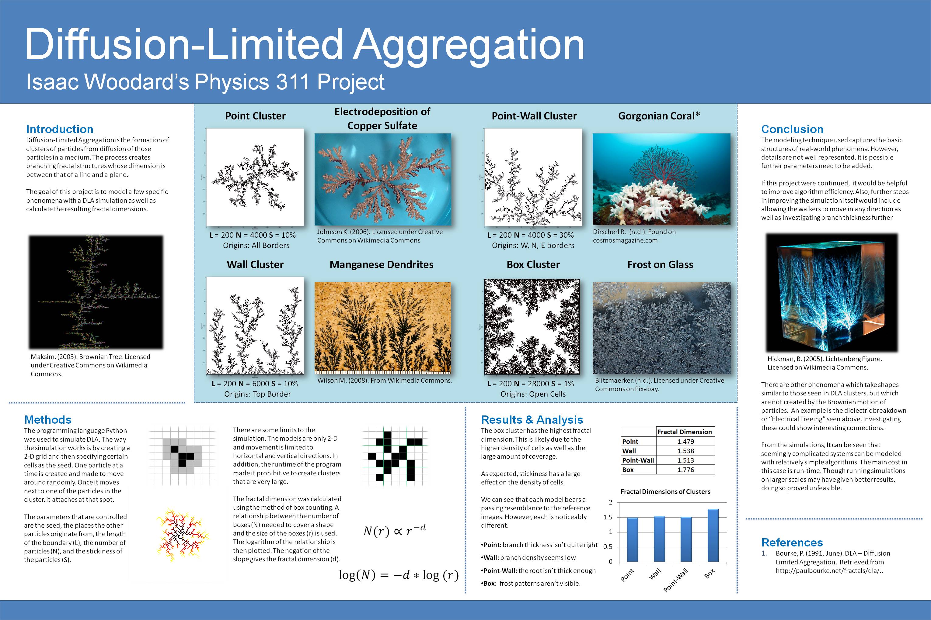
Before modeling the diffusion process, the simulation is fed a 2D grid. Some of the cells in the grid are filled to function as the seed. The black cells in the grid to the right represent the seed.
At this point, the simulation starts creating one particule at a time and moving it horizontally or vertically in the grid until it encounters a filled cell. This is also known as a random walk and the moving particle is called the random walker. "Encountering" a filled cell means entering an adjacent or diagonal cell, shown as grey in the diagram.
When the random walker encounters a filled cell, one of two things can happen depending on the value of the sticky coefficient. If the coefficient is 1, the walker will stick and become part of the cluster. If the coefficient is less than 1, the walker may continue moving rather than sticking to the cluster.
Cluster Shape & Parameters
The shape of the cluster is primarily determined by the location and shape of the seed, the possible starting locations of the walkers, and the sticky coefficient S. The diagrams on the left display the age of each cell in the cluster, with black being the oldest and yellow the youngest. We can see the walkers are unlikely to reach the inner branches as the cluster grows in size.
The other two parameters are the length of the grid boundary L and the number of walkers N. Increasing the size of the grid has a large impact on the runtime of the algorithm since each walker has to encounter the cluster to stick. In contrast, adding additional walkers has a small effect on the runtime because it is easier to encounter the cluster as it grows larger. However, adding too many walkers oversaturates the cluster and damages the fractal pattern.
There are some limits to the simulation. The grid is 2D rather than 3D and movement is restricted to horizontal and vertical directions. In addition, the runtime of the program made it prohibitive to create larger clusters than those shown.
Calculating the Fractal Dimension
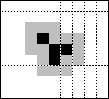
The fractal dimension of the clusters was calculated using the Minkowski dimension, also known as the box-counting method.
Using this method, the cluster is covered in squares of the smallest possible size. The number of squares is proportional to the inverse of r raised to the power of the fractal dimension d. We can take the logarithm of the relationship and solve for the fractal dimension.
Typically, the number of squares is found for multiple square sizes as the algorithm searches for the smallest possible size. This gives a set of values which can be plotted on a log graph with the slope being the negation of the fractal dimension.
N(r) ∝ r-d → log N = -d × log r
Results
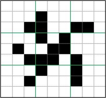
The minimum fractal dimension of the clusters was 1.479, indicating they do indeed have significant fractal properties.
Despite differences in parameters, the Point, Wall, and Point-Wall Clusters had similar fractal dimensions. The Box Cluster was noticeably different, perhaps because of the extreme number of walkers and low stickiness. We can see the impact of stickiness on branch thickness by comparing the Box Cluster to the others.
The initial parameters were tweaked to create a structure resembling the reference images. However, there are some visible differences:
- Point: branch thickness isn't quite right.
- Wall: branches are less tightly packed.
- Point-Wall: the thickness of the root is the same as the branches.
- Box: the sharpness of the frost pattern is absent.
Reflection
The DLA simulation did a good job of capturing the basic structure of the real-world phenomena and could be seen as a rudimentary way to approximate their fractal dimensions. Modeling the phenomena more accurately would likely require more walkers in a larger grid or additional parameters, such as making stickiness a function of distance from the seed. Allowing diagonal movement might also have an impact on how the clusters form.
It would be interesting to adapt the simulation to 3D. There were practical limitations keeping me from considering that for the this project. While it might not have been much more difficult to code, the clusters would have been more difficult to display on a poster. It also would have increased the hardware demands, and at the time I was trying to get everything to run on my laptop...not the wisest of choices in hindsight.